A Comparative Data Analysis of Eliud Kipchoge’s World Record at the 2018 Berlin Marathon
A Brief Overview
In the time since Eliud Kipchoge’s Breaking2 attempt on the Monza race-track in Italy, which secured him a place in the history books with 2 hours and 25 seconds over the marathon distance, he has seemed inevitable that he would go on to break the current marathon world-record, secured held by [Denis Kimetto] (https://www.iaaf.org/news/report/marathon-world-record-dennis-kimetto-berlin) since 2014 with a time of 2:02:57. And so, as Sunday morning approached the talk seemed less about if the current world-record would fall, and more about by how much.
Since 1998 there have been 7 new male marathon world-records set on Berlin’s fast and flat course, 3 of them since 2010. Would we see a another? Sure enough, as if to order, Eliud Kipchoge served the latest world-record to Berlin crowds, crossing the line in an incredible 2:01:39, smashing the previous record by 1 minute and 18 seconds; we haven’t seen a record breaking margin of more than a minute since Derek Clayton lowered the world record from 2:12:00 to 2:09:37 in 1967; which is currently ranked 1,203 in the world. It was all the more impressive because the 33-year-old Kenyan achieved it while running the last 17km on his own after the last of his pacers, not to mention the rest of the field, drifted away long before the finish.
sub_210 %>%
  filter(runnier == "Derek Clayton") %>% pull(rank)
## [1] "1203" "2212"2:01:39 in Comparison
How does Kipchoge’s new record compare with previous WRs? The great thing about Berlin is that it attracts the best of the best and so not surprisingly quite a few WRs have been established there. This means we can perform a like-for-like comparison by comparing Kipchoge’s race to (in our dataset) the previous 5 fastest times in Berlin:
#' AN INTERATIVE TO SHARE RESULTS MAYBE BASED IN SHINY ...
top_times %>% arrange(rank) %>%
  filter(str_detect(marathon, "Berlin")) %>%
  head(5) %>%
knitr::kable()| rank | runner | home | marathon | km_5 | km_10 | km_15 | km_20 | km_21.1 | km_25 | km_30 | km_35 | km_40 | km_42.2 |
|---|---|---|---|---|---|---|---|---|---|---|---|---|---|
| 1 | Eliud Kipchoge | Kenya | Berlin 2018 | 00:14:24 | 00:29:01 | 00:43:38 | 00:57:56 | 01:01:06 | 01:12:24 | 01:26:45 | 01:41:01 | 01:55:32 | 02:01:39 |
| 2 | Dennis Kimetto | Kenya | Berlin 2014 | 00:14:42 | 00:29:24 | 00:44:10 | 00:58:36 | 01:01:45 | 01:13:08 | 01:27:38 | 01:41:47 | 01:56:29 | 02:02:57 |
| 3 | Kenenisa Bekele | Ethiopia | Berlin 2016 | 00:14:21 | 00:29:00 | 00:43:37 | 00:58:02 | 01:01:11 | 01:12:47 | 01:27:30 | 01:42:01 | 01:56:55 | 02:03:03 |
| 5 | Wilson Kipsang | Kenya | Berlin 2016 | 00:14:20 | 00:29:00 | 00:43:37 | 00:58:02 | 01:01:11 | 01:12:47 | 01:27:26 | 01:41:56 | 01:56:56 | 02:03:13 |
| 6 | Emmanuel Matai | Kenya | Berlin 2014 | 00:14:42 | 00:29:24 | 00:44:09 | 00:58:35 | 01:01:46 | 01:13:08 | 01:27:37 | 01:41:48 | 01:56:36 | 02:03:13 |
Figure 2 shows the pacing (in decimal mins/km) for all 4 WRs across each of the 5km segments of the race (5 km, 10 km, …, 40km), and the final 2.195km segment. In each case the dashed line reflects the average pace for the runner in question. Based on the timing data released by the Berlin Marathon, Kipchoge ran the first 5 km in 14 mins, 24 seconds, or anout 2:53 mins/km, and he ran between 2:52 mins/km and 2:56 mins/km until the final 2.195 km stretch, which he dispatched at just under 2:48 mins/km pace, faster than any of last three male WRs managed in Berlin.
berlin_top <- top_times %>% arrange(rank) %>%
  filter(str_detect(marathon, "Berlin")) %>%
  #' WE CAN ADD MORE RUNNERS IF WE CAN GET ALL THE PLOTS TO BE SIDE TO SIDE
  #' ELIUD HAS TWO RECORDS IN THE TOP 6
  slice(c(1:5,7)) %>% select(rank) %>%
  inner_join(top_times_splits, by = "rank") %>%
  mutate(runner = factor(runner, levels = berlin_best))

berlin_top %>% select(runner, split_num, distance_ran, seconds_split) %>%
  #' CALCULATE ESTIMATED PACE
  pace_calculator(distance = "distance_ran",
                  metric = "km",
                  seconds = "seconds_split") %>%
  #' CALCULATE OVERALL PACE
  group_by(runner) %>%
  mutate(overall_pace = sum(seconds_split) / 26.2,
         overall_pace =
           as.numeric(paste(trunc(overall_pace / 60),
                            round(overall_pace %% 60), sep = "."))) %>%
  ungroup() %>%
  #' VISULIZATION OF SPLITS
ggplot(aes(split_num, mi_pace)) +
  stat_mean_line(color="red", aes(split_num, overall_pace)) +
  geom_point() +
  scale_x_discrete(breaks=c(10, 20, 30, 40)) +
  #' IT WOULD BE NICE FOR THE RUNNIER TO BE RANKED IN DISTANCE
  facet_wrap(~ runner, ncol = 6) +
   labs(title = "Berlin's Top Runners",
       subtitle = "Figure 1 - Less than 3 Seconds Per Mile Distinguishes the World's Best Marathoners",
       x = "Kilometer Splits",
       y = "Per Mile Pace") +
  pretty_theme_avg_pace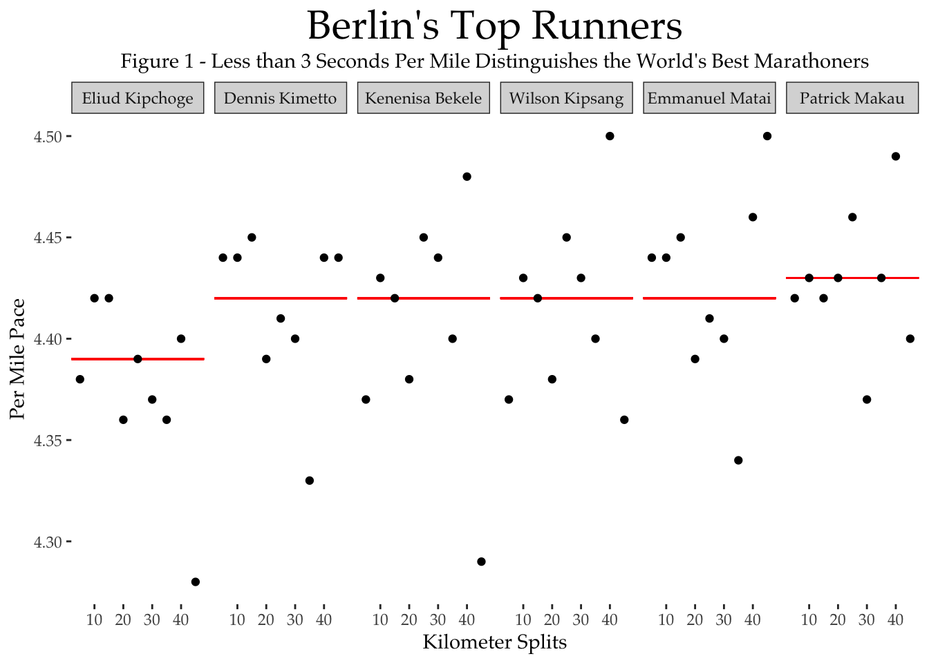
2:01:39 by the Splits
Kipchoge, and Kimetto before him, secured their world-records with negative splits, running the second half of the race more than 30 seconds faster than the first half. In contrast Kipsang and Musyoki secured their records with slight positive splits, running the second half about 10 seconds slower than the first; see Figure [X]. Since 2010 about half of the Berlin winners have run negative splits, averaging a 30-second difference, and half have run a positive split, averaging a 45-second difference.
top_times %>% arrange(rank) %>%
  filter(str_detect(marathon, "Berlin")) %>%
  #' WE CAN ADD MORE RUNNERS IF WE CAN GET ALL THE PLOTS TO BE SIDE TO SIDE
   slice(c(1:5,7)) %>% select(rank) %>%
  inner_join(top_times, by = "rank") %>%
  mutate(runner = factor(runner,
                         levels = berlin_best)) %>%
  mutate(
  first_half = as.numeric(km_21.1),
  second_half = as.numeric(km_42.2 - km_21.1),
  half_split = second_half - first_half
  ) %>%
  #' HISTOGRAM OF NEGATIVE SPLITS
  ggplot(aes(runner, half_split)) +
  geom_bar(stat = "identity", aes(fill = runner), legend = FALSE) +
  geom_text(aes(
  label = paste(half_split),
  vjust = ifelse(half_split >= 0, 0, 1)
  )) +
  scale_y_continuous() +
  theme(
  axis.title.x = element_blank(), #' REMOVES RUNNER FOR THE AXIS TITLE
  axis.text.x = element_blank(),  #' REMOVES NAMES FROM THE X AXIS
  axis.ticks.x = element_blank()  #' REMOVES THE DASHES
  ) +
  # MODIFY LEGEND TITLES
  labs(title = "Berlin's Top Runners",
       subtitle = "Figure 2 - Kipsang, the King of Positive Splits",
       x = "",
       y = "Half Split (Seconds)") +
  scale_fill_manual(values=c("#0062B4FF", "#0062B4FF", "#FF4C4CFF", "#FF0000FF", "#4883B4FF", "#FF9999FF")) +
  pretty_theme
## Warning: Ignoring unknown parameters: legend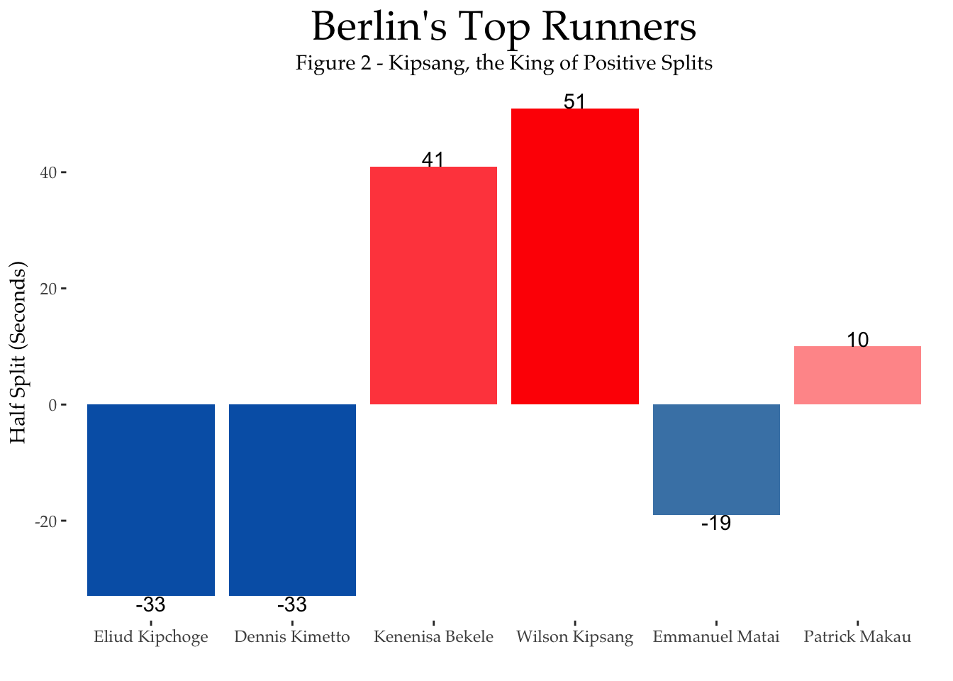
2:01:39 from Behind
Finally, let’s replay these five Berlin WRs in the same (virtual) race, to get a better sense of how the lead pack might have looked had these incredible runners toed the line together at the height of their performance, to run their WR races. Obviously we cannot account for the additional competitive tension that this might have introduced, but we can at least compare their pacing and timing information to get a better sense of how this lead pack might have developed.
  berlin_top %>%
  select(runner, split_num, time) %>%
  #' CREATE A PROPER COLUMN NAME
  mutate(runner = str_replace_all(runner, " ", "_")) %>%
  spread(runner, time) %>%
  select(split_num, Eliud_Kipchoge, everything()) %>%
  #' DEVELOPE A VIRTUAL RUNNER THAT RUN AN EVEN WR PACE
  mutate(Virtual_Runner =
           round(
           (period_to_seconds(hms("2:01:38")) / 42.195) *
           as.numeric(as.character(split_num)))) %>%
  #' TAKE THE DIFFERENCE OF A RUNNER SPLIT COMPAIRED TO WORLD RECORDS PACE
  mutate_at(.vars = str_replace_all(berlin_best, " ", "_"),
            funs(!! .$Virtual_Runner - .)) %>%
  #' THE VIRTUAL RUNNER SHOULD ALWAYS BE ON WR PACE
  mutate(Virtual_Runner = 0) -> berlin_wr_pace


berlin_wr_pace %>%
  gather(-split_num, key = "runner", value = "second_to_wr") %>%
  mutate_at("runner", ~ str_replace_all(.,"_", " ")) -> berlin_wr_pace_long

berlin_wr_pace_long %>%
  mutate(runner = factor(runner, levels = c("Virtual Runner", berlin_best))) %>%
  ggplot(aes(x = split_num, y = second_to_wr, group = runner)) +
  geom_line(aes(linetype = runner)) +
  geom_point() +
  labs(title = "Seconds Behind a World Record",
       subtitle = "Figure 3 - Kipchoge Seperates Himself from the Virtual Pack After the Half Marathon",
       x = "Kilometer Split",
       y = "Seconds to a World Record") +
  labs(linetype = "Runner") +
  pretty_theme_seconds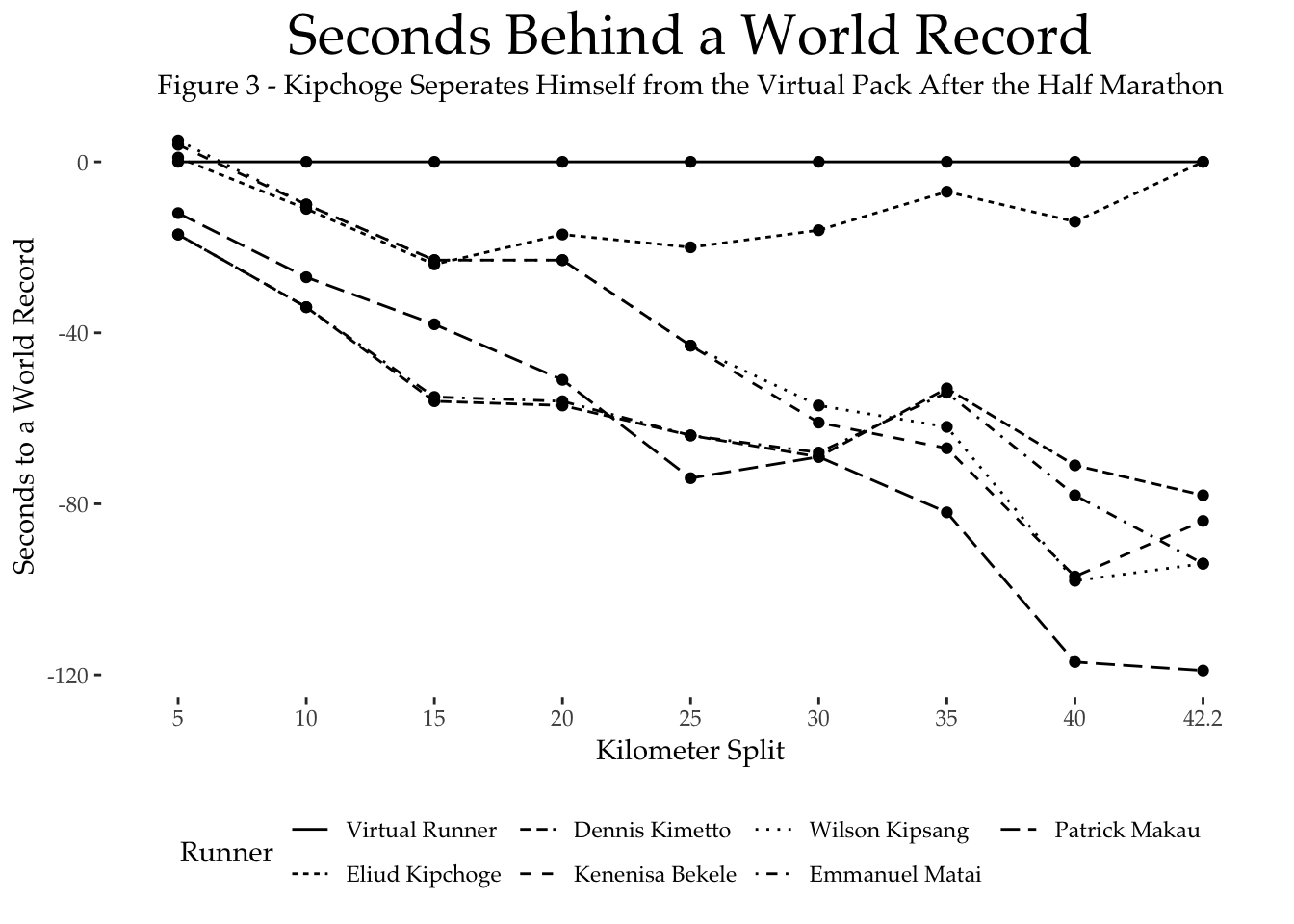
Using Kipchoge’s WR run as the baseline, Figure 6 shows the number of minutes each recent world-record holder was behind Kipchoge at the end of each 5 km race segment (and at the finish-line) in this virtual race. Kipchoge leads from the start, stays in front, and gradually but steadily extends his lead after the 15km mark. Kipsang stays in touch with Kipchoge during the first 15km of the race, getting to within just over 7 seconds by the end of the 15 km mark. But after this, begins to drop back. Meanwhile, Kimetto, after spending the first 20 km in 4th position (by 20 km he is 40 seconds behind Kipchoge), moves into second place and starts to recover some ground to get within 35 seconds of Kipchoge by the end of 35 km. Despite the beginnings of what might have been a late surge by Kimetto, Kipchoge is too strong and extends his now unassailable lead all the way to the end, finishing a full 78 seconds ahead of Kimetto, just over 94 seconds ahead of Kipsang, and almost 119 seconds ahead of Musyoki. To put this another way, we can estimate how far behind (in distance rather than time) each of Kimetto, Kipsang, and Musyoki would have been when Kipchoge crossed the line, based on their average race paces. The results of this are shown in Figure 7: Kimetto would have finished 446m (almost half a kilometer) behind Kipchoge; Kipsang would have been just under 600m behind; and Musyoki would have been 675m back. Not even even close!
berlin_mps <- berlin_top %>%
  group_by(runner) %>%
  summarise(finishing_time = max(time),
         mps = 42195 / finishing_time) %>%
  ungroup() %>%
  select(- finishing_time)


  berlin_wr_pace_long %>%
  filter(runner != "Virtual Runner") %>%
  mutate(runner = factor(runner, levels = berlin_best)) %>%
  left_join(berlin_mps, by = "runner") %>%
  filter(split_num == "42.2") %>%
  mutate(meter_to_wr = second_to_wr * (-mps)) %>%
  ggplot(aes(x = fct_rev(runner), y = meter_to_wr, fill = meter_to_wr)) +
  geom_bar(stat="identity") +
  scale_fill_continuous(low = "#FFCCCCFF", high = "#FF2626FF") +
  labs(title = "Meters to a World Record",
       subtitle = "Figure 4 - On a 400 Meter Track, Kipchoge would have Lapped the World's Best",
       x = "Runner",
       y = "Meter to a World Record") +
  coord_flip() +
  pretty_theme_meters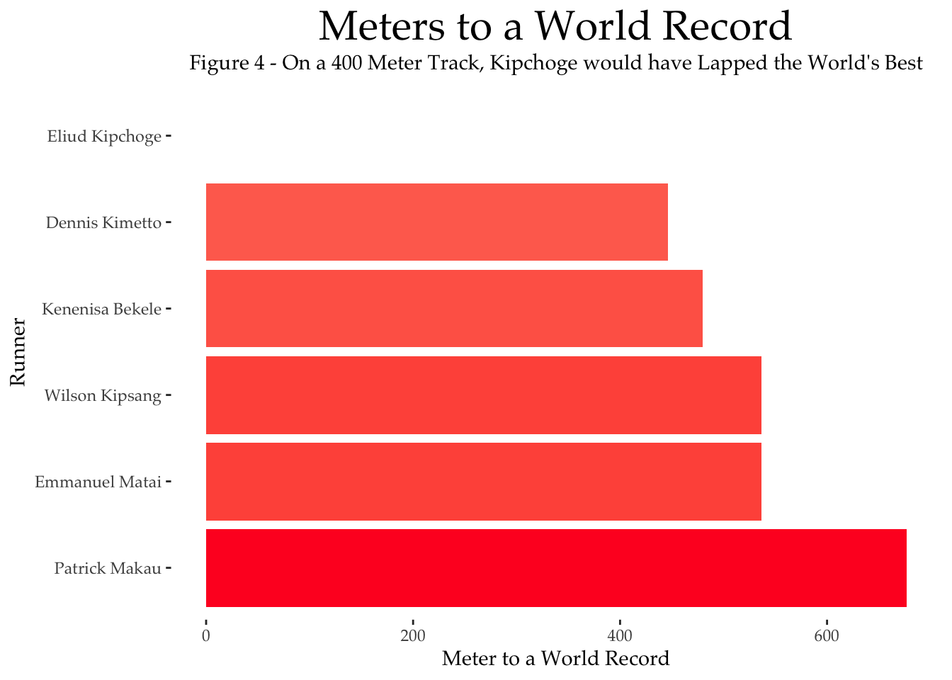
By any objective measure Kipchoge’s Berlin world-record race was nothing short of stunning. He obliterated Kimetto’s 2014 record, set on the same course, and his incredibly disciplined negative split is all the more impressive because he did it largely on his own, after dropping the last of his pacers shortly after the halfway point. It seems right and proper that on September 16th 2018 the fastest marathoner also ran the fastest marathon.